What Is Bayesian Inference?
Understanding the Concepts and Applications of Bayesian Inference in Probability Theory

Understanding the Differences between Frequentism and Bayesianism
In the world of statistics, there are two prominent schools of thought: frequentism and Bayesianism. While both approaches aim to make sense of data and the world around us, they fundamentally differ.
Frequentism is the more traditional approach, which defines probability as the limit of the relative frequency of an event as the number of trials approaches infinity. In other words, frequentists rely on the idea of repeating an experiment an infinite number of times to determine the probability of an event.
On the other hand, Bayesianism is a more modern approach that defines probability as a measure of subjective belief. Bayesian statisticians use Bayes’ theorem (more on this later) to update prior probabilities based on new data, meaning that they incorporate pre-existing knowledge or beliefs to interpret the data.
Frequentism vs. Bayesianism
a. One of the key differences between the two approaches is their interpretation of probability. Frequentism views probability as an objective property of the world, while Bayesianism sees it as a reflection of personal belief.
Frequentism is often used in experimental settings with a clear, repeatable process. In contrast, Bayesianism is used in situations where prior knowledge or belief is important or where the experimental process may be more complex.
b. Another important difference between the two approaches is their treatment of parameters. Frequentism treats parameters as fixed and unknown, whereas Bayesianism treats them as random variables with a probability distribution. This means Bayesianism is more flexible and can handle a wider range of statistical problems.
An example
Let’s assume that a company wants to estimate the probability of a new product's success in the market.
In the Frequentism Approach: The company would conduct a large number of market surveys or focus groups, collecting data on potential customers’ preferences, interests, and willingness to buy the product. Based on that, they would calculate the proportion of people who would buy the product, and that proportion would be the estimate of the probability of success.
In the Bayesianism Approach: The company would start with a prior belief about the probability of success, based on their experience and any other relevant information. As they collect data, they would update their belief using Bayes’ theorem, taking into account the prior belief, the likelihood of the data given that belief, and the probability of the data in general. The updated belief would be the estimate of the probability of success.
Both the frequentist and the Bayesian collect data from potential customers when inferring, but the Bayesian also incorporates prior knowledge about previous products' success probability.
Bayes’ theorem
Bayesian inference is a statistical technique that updates probability estimates based on new data. It is based on Bayes’ theorem, which describes the relationship between the probability of an event and the evidence that may affect it.
It is named after Thomas Bayes, an 18th-century mathematician.
The theorem states that the probability of event A given evidence B is equal to the probability of evidence B given event A, multiplied by the prior probability of A, divided by the prior probability of B.
In equation form, Bayes’ theorem is written as:

where,
P(A|B) = probability of A given B,
P(B|A) = probability of B given A,
P(A) = prior probability of A, and
P(B) = prior probability of B.
An example
Let’s say we want to determine the probability that a person has a certain disease based on the results of a diagnostic test.
We know that the test has a sensitivity of 95% (i.e., it correctly identifies 95% of people who have the disease) and a specificity of 90% (i.e., it correctly identifies 90% of people who do not have the disease).
We also know that the disease is relatively rare, occurring in only 1% of the population.
Using Bayes’ theorem, we can calculate the probability that a person has the disease given a positive test result:

= 0.95 * 0.01 / (0.95 * 0.01 + 0.1 * 0.99)
= 0.086 or 8.6%
This means that even if a person tests positive for the disease, there is still only an 8.6% chance that they actually have it.
The basic idea behind Bayesian inference is that probabilities can be thought of as degrees of belief and these degrees of belief can be updated as new information becomes available.
How does it begin?
Bayesian inference begins with an initial prior probability distribution, which expresses a person’s beliefs about the probability of an event before any data is collected. As new data is collected, the prior probability distribution is updated using Bayes’ theorem, which describes how to update probabilities based on new evidence.
One of the key advantages of Bayesian inference is its ability to incorporate prior knowledge into statistical analyses, leading to more accurate results, especially when data is limited or noisy. However, this also means that the results can be sensitive to the choice of prior probability distribution and researcher has to be mindful about choosing an accurate prior probability distribution.
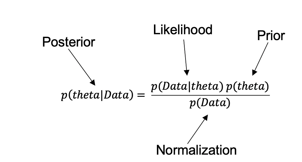
Parameters of Bayesian Inference Theorem

- Likelihood refers to the probability of observing the data, given a specific value of the parameter. This is a function of the data and the parameter, and it is often denoted as p(Data|Theta).
- Prior refers to the probability distribution of the parameter before we observe any data. It is denoted as p(Theta), and it represents our prior beliefs or knowledge about the parameter.
- Posterior refers to the probability distribution of the parameter after we observe the data. It is proportional to the product of the likelihood and the prior and is denoted as p(Theta|Data). After observing the data, the posterior distribution represents our updated beliefs or knowledge about the parameter.
- Normalization refers to the integration of posterior distribution and is done by dividing the product of the likelihood and the prior by a normalizing constant. It is indirectly proportional to posterior and is denoted by p(Data).
- Prediction error refers to the discrepancy between the observed data and the predicted data based on the model. It is often used to evaluate the performance of a Bayesian model, and it is calculated as the difference between the observed data and the expected value of the predicted data.
I appreciate you and the time you took out of your day to read this! You can find more articles like this from me on QuickGuide blog. For news and insights, please find me on Twitter at @osheenjain, to see what I do when I’m not working, follow me on Instagram.
Don’t forget to like and subscribe on Medium, this motivates me a lot!
